Data Source

There are four ways you can display the source data for a chart.
1) Displaying the Select Data dialog box.
2) Using the Chart Range Indicator you can quickly see which range of cells an embedded chart is referring to.
3) Seleting an individual series and editing the Series Formula.

The quickest way to selected stuff is to use the Layout tab at the top
Select Data Source dialog box

Add - Displays the Edit Series dialog box explained below allowing you to select the data from a new series
Edit - Displays the Edit Series dialog box explained below
Remove - Removes the series which is currently selected

Hidden and Empty Cells -

Edit Series dialog box
Lets you change the Series name and the Series values

Chart Tools, Design Tab

When you activate a chart the contextual Chart Tools tabs are automatically displayed.
You can display the source data for the active chart by activating the chart and selecting Select Data.
This will display the Select Data dialog box.
SS - Select Data

Using the Chart Shortcut Menu

The easiest way to adjust the source data of a chart is to right mouse click and select "Source Data" and click on the series tab.
You can select either the chart area or the plot area to display this shortcut menu.
SS - plot area shortcut menu

Using the (Chart > Source Data) dialog box

Displaying the (Chart > Source Data) dialog box gives you much greater control over the indidiual series on your chart.
You can modify the range reference on the Data Range tab to adjust the data range for the whole chart.
The Data range textbox displays the range of cells which is being used for the source data.
If you originally selected a single cell, then this will have been automatically expanded to the current region.

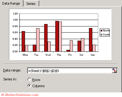Data range - You can edit the cell range manually or you can use the mouse to highlight a different range. Using the arrow keys while in this box will actually select cells instead of moving your position within the box.
Rows - Plots the data series of the chart using each row as a separate series.
Columns - Plots the data series of the chart using each column as a separate series.

You can modify the range references for the individual series using the Series tab of this dialog box.

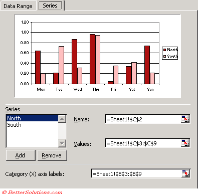Series - The series list displays the names of all the data series on the chart. Selecting a particular series will display the corresponding Name and Values.
Add - Adds a new data series to the active chart.
Remove - Removes the currently selected series from the active chart.
Name - This is used in the Legend to identify the series.
Values - These are the data series values.
Category (X) axis labels - These are chart specifc and not series specific. If there is no category axis labels provided then a list of sequential numbers will be used.

Your source data can use named ranges instead of direct cell references

Delink Chart

Series - press F9 in the Formula Bar
VBA - for each series
myseries.XValues = myseries.XValues
myseries.Values = myseries.Values
myseries.Name = myseries.Name

peltiertech.com/Excel/ChartsHowTo/DelinkChartData.html

Remember

The Automatic Range Finder can only be used with embedded charts when the chart is on th same worksheet as the data.
If you delete the source data for a chart and press F9 your source data will contain #REF's and will have to be re-defined.
Source Data in hidden rows is not shown by default but you can change the setting (Tools > Options)(Chart tab, "Plot Visible cells only").
It can sometimes be easier to overwrite the series name which will typically be a cell reference just to a hard types string constant contained in double quotes.
If a whole chart is selected then the "Data Range" tab will be displayed by default when you display the Source Data dialog box.
If an individual series is selected then the "Series" tab will be displayed by default when you display the Source Data dialog box.

Switch Row Column

Range Indicator

Also known as the Chart Range Finder.
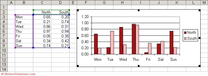
When you activate a chart the source data will be automatically highlighted when the data range is not too complex.
This method can only be used with embedded charts when the chart is on the same worksheet as the data ?
When the chart area is selected its source data will be highlighted.

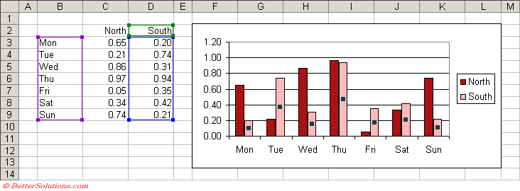
When an individual series is selected its source data will be highlighted.

If you select the chart, instead of a series all the series are outlined in one colour and the series labels in another.
If you select a series, the series is in one colour and the series category labels are in a different colour.
When you edit a series formula, the cells and ranges that the formula refers to is outlined in one colour and the series category labels in a different colour.
Selecting an individual data series will highlight only the source data for that specific series.
The range of cells consists of one or more coloured ranges.
Purple - Series labels (X-axis) or categories
Blue - Values (Y-axis)
Green - Bubble Sizes / Series name, Legend details
Each outline has a handle (i.e. a small square in the bottom right corner) and the source data can be increased or decreased by dragging this handle.
Each of the highlighted ranges contains a small handle in each corner which can be easily dragged to expand or reduce the range used for the source data.
The source data can even be moved by selecting the edge and dragging the outline.
It is possible to extend the range of cells within your source data and see the chart updated immediately including the new data.
Changing values are reflected immediately.
Note that the data for an individual data series must be continuous. The colour cannot be changed.
You can alternatively just drag the source range indicators and fill handles.
A way to update your charts (i.e. re-link / assign the source data) without to press F9 which updates the whole worksheet
You can extend the ranges by placing your mouse at the corner of the data range. You should see the pointer turn into a small plus sign, press down and drag the mouse until the coloured border extends to include the new cells. Release the mouse and the chart will update.

Use the handles to drag expand or contract the range
Drag the whole range to different cells
Only works with embedded charts, not chart sheets

Changing the Source Data

It is also possible to use the Automatic Range Indicator to adjust the data ranges.
Marching ants border around the cell range(s).
This method is often the quickest and easiest.
It is possible to adjust the whole range or just an individual series by dragging the broder or the square in the bottom right corner.
You can even drag one of the sides to move the whole data block in one go.
For more information about the automatic range finders, please refer to the previous page.

Excel 2007 Changes

You can no longer drag a range of cells onto a chart to include more series. Instead you can copy the cell range and paste onto the chart.
You can no longer drag individual data points to automatically change the source date.
Legend - any series that does not have a name will appear in the legend as "series1", "series2" etc
2007 - blank rows when you have a date x-axis - seems to default to the first date on the axes (and not even zero).

Hidden and Empty

These settings only apply to the active chart and applies to all the series on the chart
All the series must have the same cell settings

This dialog box can be accessed from the Select Data Source dialog box.
Office Article - Display hidden worksheet data and empty cells in a chart, Interpolating missing values - KB 214096

This settings only applies to some of the chart types:
Line, XY Scatter and Radar charts
For all other chart types, missing data is simply not plotted - CHECK THIS
SS

You can force Excel to interpolate by putting =NA() in the necessary cells ?

Plot Visible Only

Usually Excel doesn't plot data that is in hidden rows or columns
To override this remove the checkmark from this option
This setting is chart specific

Changing

There are five ways you can change the source data of a chart.
Overwriting the cells with different values.
Using the Select Data dialog box.
Using the Range Indicator.
Editing the Series Formula.
Dragging individual Data Points.

Overwriting the Cells

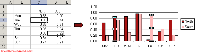
When a chart is created the source data is linked to the chart object meaning that any changes to the data are reflected on the chart automatically.
Lets change the values in cells "C4" and "D7" to 0.85 and 0.92 respectively.

Dragging individual Data Points

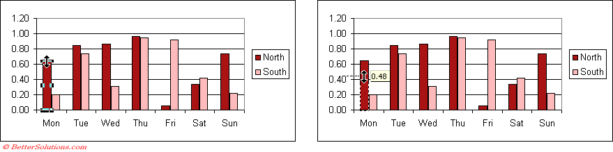
You can also drag the chart data point to change the value on the worksheet.

Adding Source Data / Series

The series tab - You can use the Add button to create a new series and the Remove button to remove any
You can modify these ranges either by editing the range directly or by dragging the automatic range finders

The Source data dialog will change slightly if a bubble chart is activate

All the data for a specific series must be on the same worksheet. It does not have to be in a contiguous range. You can use data from different worksheets on the same chart by using different series. Step 2, Series tab ot the Chart Wiward.
A bubble chart requires an additional set of data to define the size of the bubbles.

Adding a Series

Select the cells containing the new data series (Edit > Copy). Click the chart and select (Edit > Paste). It will either be added immediately or the Paste Special dialog box will be displayed.

Removing a Series

You can easily remove a data series from a chart by selecting it and pressing Delete.
You can alternatively select (Edit > Clear > Series).

A surface chart does not let you select a specific series ??

Adding More Data

After you have created a chart you can very easily add another data series to it. Select the cells containing the new data series, copy the data, select the chart and paste the data.
There are several ways you can add an additional series to an existing chart.
1) Select the chart area and drag the colour range markers to include the additional cells.
2) Select the new cells and copy them to the clipboard. Select the chart and paste the data on top of it.
3) Select the new cells and drag them on to the chart.
If you need to plot data that is on more than one worksheet, you can add another series once the chart has been created.

Select the area of the new data series. (Edit > Copy). Click on the chart and (Edit :> Paste) . It will either add it straight away or it will display the Paste special dialog box
When you select the chart area it should highlight the source data automatically (colour coding) You can drag the corners to add more data. You can extend the source data, but then hide the rows. This means that the data points are not actually plotted.
To delete a series just select the series and hit delete

Avoid copying the charts as objects (white handles) and always copy them as chart objects (black handles).
If you have data with years in one column then Excel will treat this column as a data series and not as the category-axis labels

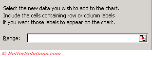
(Chart > Add Data) dialog box

If you want to plot data from different worksheets this must be done using Step 2 of the chart wizard.
You should create your chart initially using just one series of data. The additional series can the be added afterwards.

Series Formula

A data series is just a group of related data representing a row or column from the worksheet.
When you select a particular data series on a chart its corresponding series formula will appear in the formula bar.

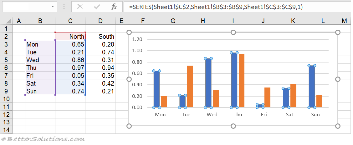When the source data is changed you will see that the series formula is changed automatically.
When a series is selected the series formula is displayed in the formula bar at the top. The name of the series is displayed in the "Name box" to the left of the formula bar.
Excel uses a series formula or function to define a data series for a chart. There is one series formula for each data series.
Although this resembles a typical worksheet formula there are a few important differences.
1) The SERIES function cannot be used directly from another cell.
2) This formula cannot contain any worksheet functions.
It is possible though to edit this formula and to manually change the arguments.

Surface charts do not have series formula ?
chart types - 83,84,85,86

[=SERIES(Name, X-Values, Y-Values, PlotOrder, Bubble Sizes) ]

The data used in each series in a chart is determined by its SERIES formula. Press Enter to apply any changes.
Name - (Optional) - This is the name of the series and is displayed in the legend. If the chart has only one series this name is used as the title. This can be blank, a text string in double quotes, a reference to a worksheet range or a named range. If this is left blank, then Excel will provide a default name (Series 1, 2, 3 etc)
X-Values - (Optional) - These are the labels that are used on the category axes. If this is left blank then consecutive integers are used 1,2,3 ... This can be blank, a literal array of numeric values or text labels enclosed in curly brackets, a reference to a worksheet range or a named range. It is also possible to have a non-continuous range reference. The separate ranges must be put inside a bracket and must be separated by commas (eg ??)
Y-Values - These are the values you want to plot. This can be blank, a literal array of numeric values enclosed in curly brackets, a reference to a worksheet range or a named range. It is also possible to have a non-continuous range reference. The separate ranges must be put inside a bracket and must be separated by a commas (eg ??).
PlotOrder - This is the plotting order for the data series. The Series tab displays the series in the order in which they are plotted. This is also the order in which the series names will appear in the legend. When there is only one series then this is omitted. This must be a whole number between 1 and the number of series on the chart. If you enter zero then 1 is used. If you enter a number greater than the number of series then the total number of series is used. This cannot be a cell reference.
Bubble Sizes - (Optional) - These are the values of the bubble sizes. This can be blank, a literal array of numeric values enclosed in curley brackets, a reference to a worksheet range or a named range. It is also possible to have a non-continuous range reference. The separate ranges must be put inside a bracket and must be separated by a commas (eg ??).

Series Formula Rules and Facts

Range references in a SERIES formula are always absolute and always contain a worksheet name. If you have defined named ranges then the series formula can contain a named range in place of a range.
Any range references used are always prefixed with the worksheet name.
Any range references used are always absolute references (as opposed to relative).
If you accidently remove the worksheet name or use a relative reference, these will be changed automatically.
Each data series has a corresponding series formula and the number of arguments will depend on the chart type.

Examples of Valid Series Formula

=SERIES(Name, X-Values, Y-Values, PlotOrder, Bubble Sizes)
=SERIES(Sheet1!$C$2, Sheet1!$B$3:$B$9, Sheet1!$C$3:$C$9, 1)
=SERIES("North", {"Mon","Tue","Wed","Thu","Fri","Sat","Sun"}, {0.65,0.21,0.86,0.97,0.05,0.34,0.74}, 1)
=SERIES(Sheet1!$C$2, , Sheet1!$C$3:$C$9, 2)
=SERIES(Sheet1!$C$2, Sheet1!$B$3:$B$9, Sheet1!$C$3:$C$9, 3, Sheet1!$D$3:$D$9)
=SERIES(, (Sheet1!$B$3:$B$9, Sheet1!$B$20:$B$30), (Sheet1!$C$3:$C$9, Sheet1!$C$20:$C$30), 4)

Changing the Arguments

You can change any of the series formula arguments in four ways you can change the series name of a data series:
1) Overwriting the cell(s) which the argument refers to.
2) Using the Automatic Range Finders to move the source data.
3) Using the (Chart > Source Data)(Series tab).
4) Editing the Series Formula.
The only way to change the order of the data series is to either use the (Chart > Source Data)(Series tab) or to edit the series formula directly.

Remember

Excel's normal practice is to assume that all the series share the same X-Values in the first column or row and that each successive column or row holds the Y-data for a separate series.
Surface charts do not have series formulas.
When you create a chart that uses a named range, Excel does not automatically substitute the name in the series formula.
If you delete a named range that is used in a chart series, the invalid name will remain and the chart will not display properly.
Pie charts can only have a single series unless .....
All the different parts of a series formula (except Plot Order) can be linked to a worksheet (in any workbook).
The maximum number of data points on a normal 2D chart is 32,000.
Bubble charts need three sets of values representing the x value, y value and the size of the bubbles.
You can display as many as 255 different data series on a chart (except Pie Charts).
Try to avoid having too many data series on a single chart.
You can have a chart object with no series, although I can't see any point
There is a direct link between the chart and the worksheet containing the data. It is possible to change the underlying data in the worksheet by dragging a individual chart point to a new position.
It is important to remember that any of the parameters in the SERIES formula can be a constant, a literal arrway a reference to a worksheet range or a named range.

Source Data Expands Automatically

If you have a data series that you add data to on a regular basis then you can easily expand the data source automatically to include the additional rows.
This method uses a combination of named ranges and worksheet functions.
In this example we want to include all the data below the headings in row 2 and for any additional data to be automatically included.
Lets use the following table of data and lets create a simple line chart.

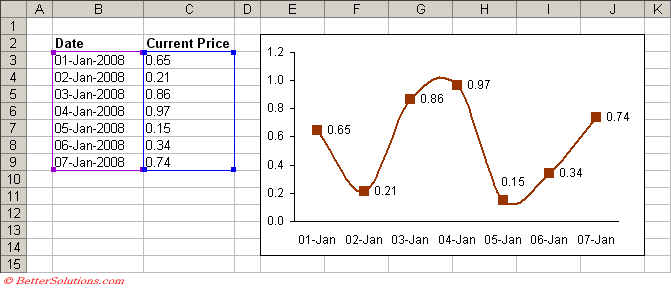Creating the Named Ranges

The named range that we need to use will have to be a Dynamic Named Range. These will change automatically.
We are going to use two worksheet functions in this named range:
The COUNTA function returns the number of non blank cells in a cell range.
This function is used to return the corresponding number of rows for the data series.
The OFFSET function is used to return the cell range which contains all the data.
Select (Insert > Name > Define) and type the name "ChartDates" in the Names in Workbook textbox.
Enter the following into the Refers To box:
=OFFSET(Sheet1!$B$3,0,0,COUNTA(Sheet1!$B$3:$B$100),1)
You do need to include the dollar signs $ otherwise the correct formula will not be used.
Select (Insert > Name > Define) and type the name "ChartNumbers" in the Names in Workbook textbox.
Enter the following into the Refers To box:
=OFFSET(Sheet1!$C$3,0,0,COUNTA(Sheet1!$C$3:$C$100),1)

Changing the Source Data

Once these two named ranges have been created you can use these for your source data instead of the actual cell ranges.
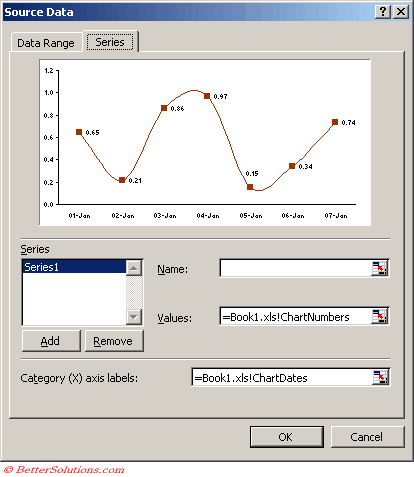
Highlight the chart, right mouse click, select Source Data and select the Series tab.
Highlight and replace the Values cell range $C$3:$C$9 with the text "=Book1.xls!ChartNumbers"
Highlight and replace the Category cell range $B$3:$B$9 with the text "=Book1.xls!ChartDates"
Any extra data you know add to your table will be automatically includes on your chart.

Remember

Be sure to include the worksheet name and there cannot be any blank rows. Do not try and type the form
For some bizarre reason you cannot use the named range "ChartValues" ?